Introduction
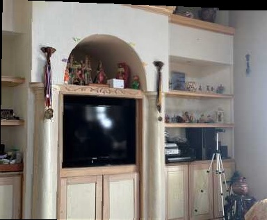
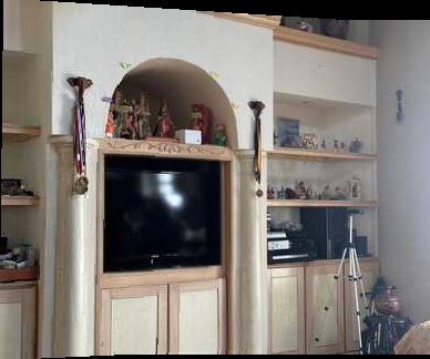
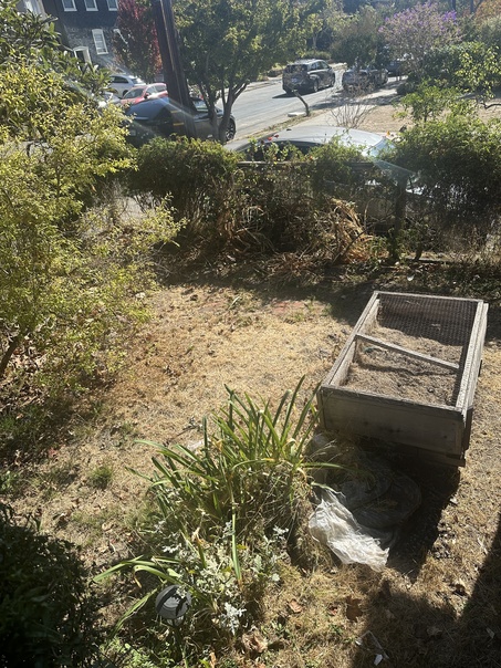
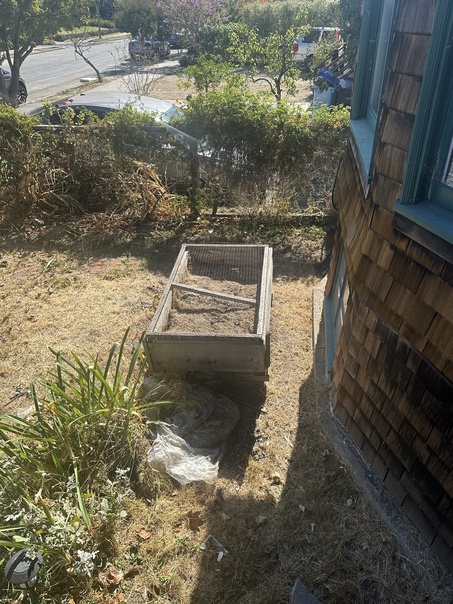
In this first part of Project 4, I learn how to warp images to other images' geographies given keypoints, as well as how to combine them into photo mosaics (panoramas)! First I get keypoints (in this part, manually), then use those keypoints to calculate the homography matrix. From there, I warp an image to another's basis, then perform Alpha-Gradient Blending to merge the images properly.
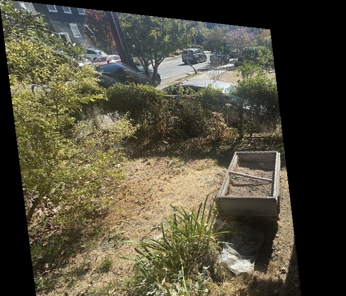
My Front Yard
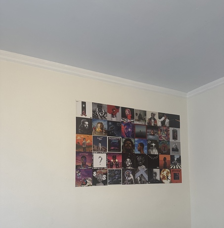
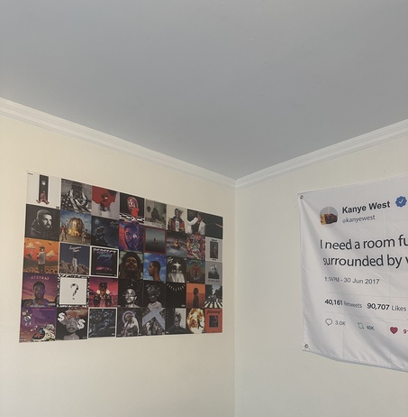
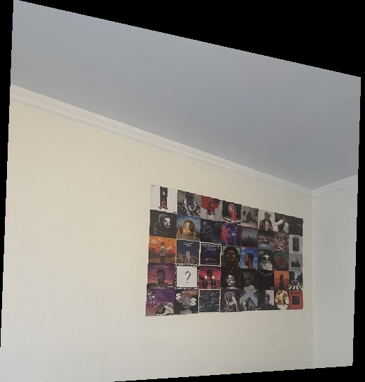
My Room
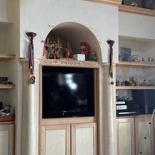
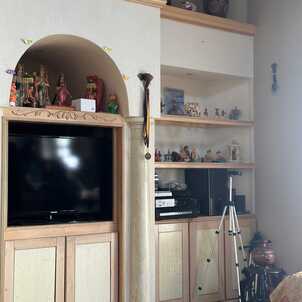
My Living Room
Recover Homographies
To align images, I need to compute the transformation between corresponding points in two images. This transformation is represented by a homography matrix H, a 3x3 matrix that relates points from one image to another via a projective transformation. Given the relationship y = H * x, where x and y are the corresponding points in the two images, I can compute the homography by solving a system of linear equations derived from the point correspondences.
Steps Involved:
- Setting up the System of Equations:
For each corresponding point pair
(x1, y1)from image 1 and(x2, y2)from image 2, two equations are generated from the projective transformation. These equations are linear in the unknown homography parameters.By stacking the equations for each point pair, I form an overdetermined system of equations A * h = 0, where A is the matrix of coefficients, and h is the vector of unknown homography parameters.
- Solving with Singular Value Decomposition (SVD):
The system of equations is solved using Singular Value Decomposition (via
np.linalg.svd), which minimizes the error in the transformation due to possible noise or imperfections in point correspondences.The result is the homography matrix H, which can be used to transform points or warp images betIen the two views.
- Reshaping the Homography:
After solving for the parameters, the homography matrix is reshaped into a 3x3 matrix. The bottom-right element is manually set to 1 (since homographies are defined up to a scale), ensuring that the matrix is correctly normalized.
Theory
The homography relates two images using the equation:
y = H * x
This implies that:
w * y1 = g * x1 + h * x2 + 1
Substituting, I get:
              (g * x1 + h * x2 + 1) y1 = a * x1 + b * x2 + c
              (g * x1 + h * x2 + 1) y2 = d * x1 + e * x2 + f
By linearizing this system, I arrive at the matrix form:
              [ x1  y1  1  0  0  0  -x2 * x1  -x2 * y1  -x2 ]
              [ 0  0  0  x1  y1  1  -y2 * x1  -y2 * y1  -y2 ]
This setup allows us to solve for the homography matrix H by stacking equations from multiple points, ensuring we have enough constraints to compute the transformation.
Warp the Images
This process involves warping one image onto another using a computed homography matrix. The homography matrix allows me to map the pixels of the source image to the perspective of the reference image, aligning them spatially. I also blend the overlapping regions smoothly using an alpha mask to reduce noticeable seams in the final merged image.
Steps Overview:
- Inverse Homography: I first compute the inverse of the homography matrix (H) to warp the coordinates of the target image back into the coordinate system of the source image.
- Extract Image Corners: I identify the corners of the source image and use the homography matrix to determine where those corners would appear in the reference image.
- Determine Output Bounds: Using the transformed corner coordinates, I calculate the minimum and maximum x and y values to determine the size of the canvas for the warped image.
- Warp Image: I create a meshgrid for the warped image, apply the inverse homography, and map valid pixels from the source image to the warped image.
- Optional Image Rectification: If the function is called with the `rectify=True` flag, only the warped image is returned. This step ensures that the two objects are aligned.
- Initialize Merged Image: If `rectify=False` I return the image mosiac combining both images. For this step, blending is needed, so I initialize a blank canvas for the merged image, which will hold both the warped and reference images.
- Blending:
- I create an alpha mask for the overlapping region, which gradually transitions from fully opaque to transparent to allow smooth blending of the images.
- Non-overlapping regions of the source and reference images are copied directly to the merged canvas.
- In the overlapping region, pixels from the source and reference images are combined using the alpha mask, creating a smooth transition between the two.
Key Concepts:
- Homography: A projective transformation that maps points from one plane to another. In this context, it transforms the source image to match the perspective of the reference image.
- Inverse Warping: To map the pixels of the warped image correctly, I apply the inverse of the homography matrix to warp coordinates back into the source image space.
- Alpha Blending: This method allows me to blend the overlapping pixels of two images smoothly, preventing visible seams where the images meet.
The result is a composite image in which the source image has been warped and blended seamlessly into the reference image, with no sharp transitions between the two.
My Front Yard

My Room

My Living Room

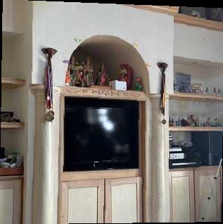
Image Rectification
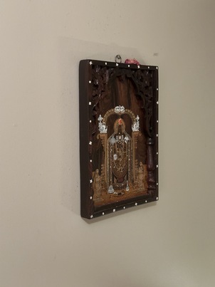
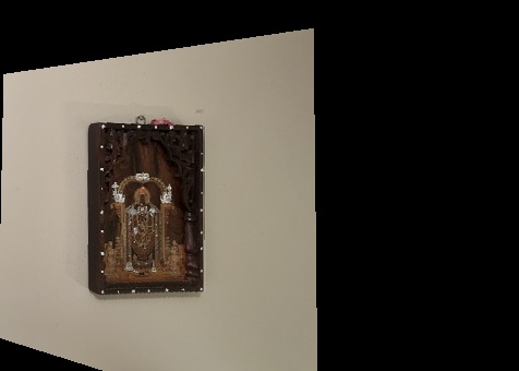
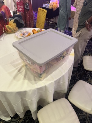
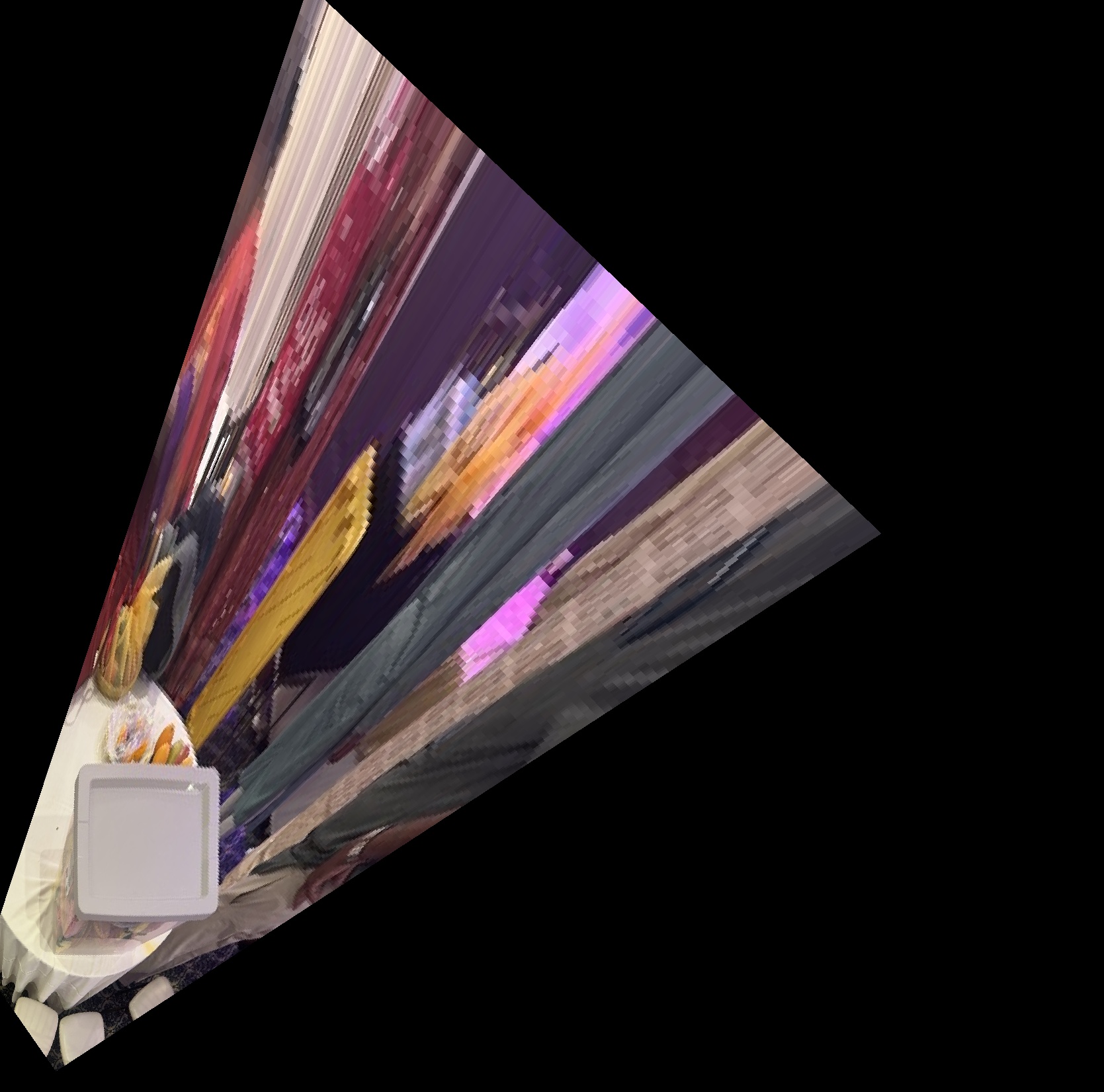
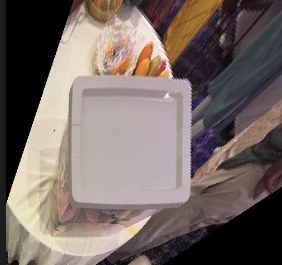
In this section, I employ the previously discussed homography computation to rectify an image, transforming a known distorted rectangular object into its proper alignment. The goal of image rectification is to warp the perspective of an object in an image (such as a painting or poster on a tilted surface) so that it appears frontal or aligned with the camera's plane of view. This is especially useful in tasks that require geometric consistency, such as 3D reconstruction, mapping, or architectural analysis.
The rectification process begins by identifying the four corner points (im1_points) of the known rectangular object in the input image. These points define the boundaries of the object before rectification. I then specify the desired output rectangle’s dimensions (im2_points), ensuring that the warped object will have the correct aspect ratio and appear undistorted.
I then compute the homography matrix H using the computeH function. This matrix captures the transformation from the input points (the distorted object in the image) to the ideal rectified rectangle. In this case, I compute the inverse homography matrix to map the original distorted points into a flat rectangle.
After computing the homography matrix, I utilize the warpImage function to warp the image based on this transformation, producing a rectified image.
Frame
Container Box
Blending Images into a Mosaic
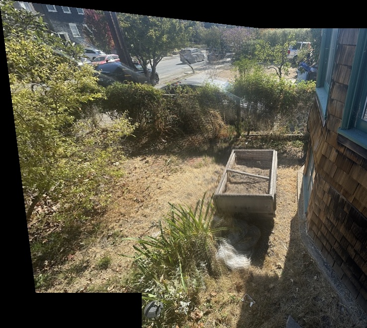
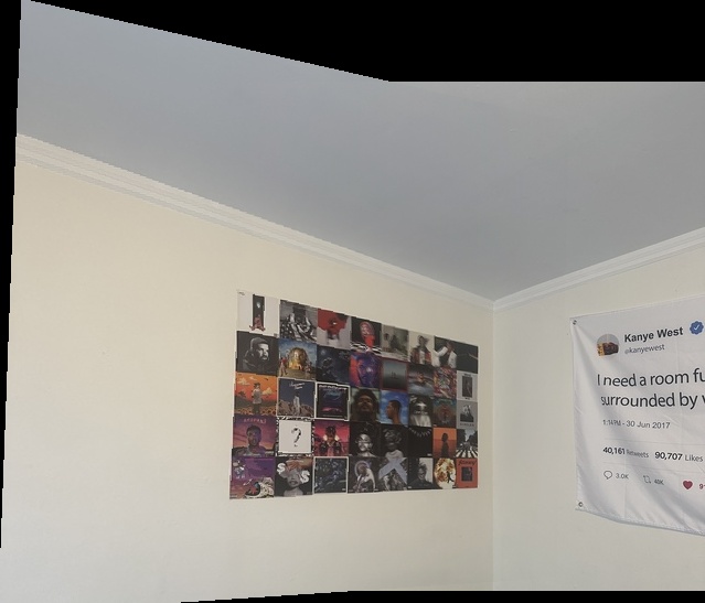
To seamlessly blend the warped images into a mosaic, I use a linear alpha gradient to ensure a smooth transition between overlapping regions. This blending technique prevents visible seams or harsh edges between the images by gradually transitioning pixel contributions from one image to another across the overlap region.
Alpha Gradient Mask Creation
The alpha mask is generated using a linear gradient that transitions smoothly across the entire overlap region. The mask starts with a value of 1 on one side (where the reference image contributes fully) and transitions to 0 on the other side (where the warped image contributes fully). This gradual change ensures a smooth blend between the two images.
Blending Procedure
Once the alpha gradient mask is created, it is applied to the overlap region. For each pixel, the reference image's value is weighted by the alpha mask value, and the warped image's value is weighted by 1 minus the alpha mask value. This results in a seamless blend without visible seams in the overlap region.
Steps in Code
- Alpha Gradient Mask Creation: A linear gradient is generated using
np.linspace. The mask smoothly transitions from one image to the other across the overlap region. - Applying the Mask: The alpha mask is applied to the overlapping region. Pixels from the warped image are weighted by the alpha mask, and pixels from the reference image are weighted by 1 minus the alpha values.
- Blending: The blended image is created using this linear gradient, resulting in a seamless transition between the two images.
My Front Yard


My Room


My Living Room


Part B: FEATURE MATCHING for AUTOSTITCHING
The second part of the project involves automatic feature matching and auto-stitching. I create a system for automatically stitching images into a mosaic. The methodology roughly follows:
- Detecting corner features in an image
- Extracting a Feature Descriptor for each feature point
- Matching these feature descriptors between two images
- Use a robust method (RANSAC) to compute a homography
- Produce a mosaic
Corner Detection
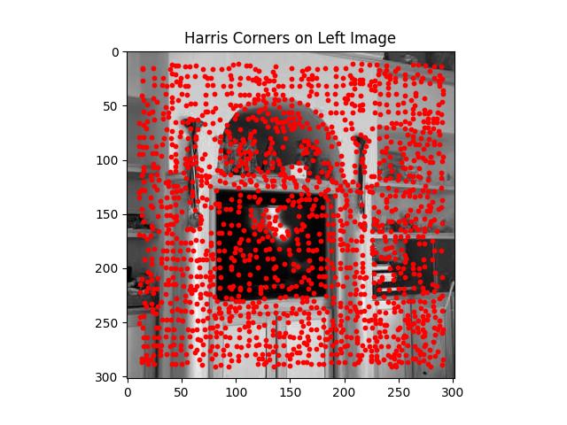
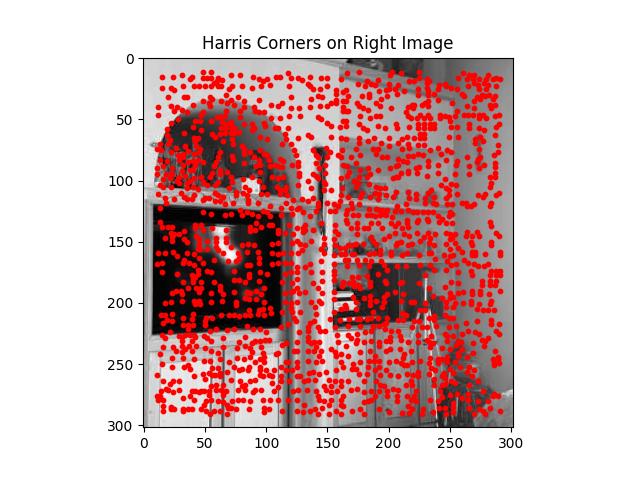
In this step, I implement the Harris Interest Point Detector to find key points or corners in an image. These key points are essential for tasks such as feature matching and image alignment, as they represent distinct points that are repeatable and consistent between images. The Harris corner detector works by identifying areas in the image where there are sharp changes in intensity in two perpendicular directions, which are typically good indicators of corners.
Below is an example of the Harris Corners for the Bedroom Picture
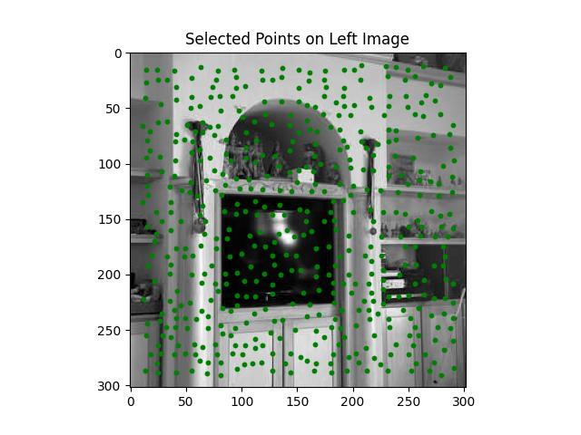
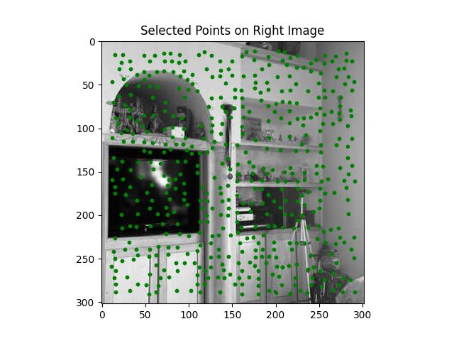
Adaptive Non-maximal Suppression (ANMS)
The Adaptive Non-Maximal Suppression (ANMS) method is used to refine a large set of detected interest points (like corners) by selecting a subset of points that are well-distributed across the image, while ensuring that the strongest points (based on their response values) are prioritized.
Key Steps in ANMS:
-
Sorting Harris Corners by Response Strength:
First, the function sorts the Harris corner points in descending order based on their response values. The strongest corner points (those with the highest response) are considered first in the selection process.
-
Initialize Suppression Radii:
For each corner, a suppression radius is calculated. This radius represents the distance between the current point and the nearest stronger point that is "sufficiently stronger" based on the threshold. Initially, the suppression radius for all points is set to infinity (
np.inf). -
Calculating the Suppression Radius:
- The function identifies stronger points (points that have a Harris response greater than the current point by a factor determined by the threshold).
- The distance from the current point to all stronger points is calculated using the
dist2()function. - The suppression radius is the distance to the nearest stronger point, ensuring that stronger points can suppress weaker ones in their vicinity.
-
Sorting by Suppression Radius:
Once all points have suppression radii, the points are sorted in descending order based on their suppression radius. This step ensures that points with large radii are prioritized, helping distribute the points evenly across the image.
-
Selecting the Final Keypoints:
Finally, the top
num_pointscorner points are selected based on their suppression radii. These points are returned as the final set of selected keypoints, ensuring that they are both strong and well-distributed across the image.
Feature Descriptor Extraction
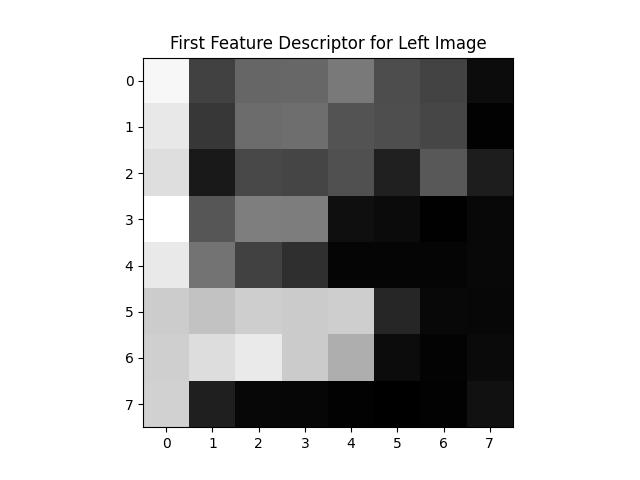
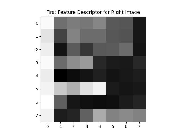
In this step, feature descriptors are extracted from keypoints detected in the image. A descriptor is a vector that represents the local neighborhood around a keypoint, allowing us to describe and compare the keypoints across different images. The extracted descriptors are used in the feature matching process to identify corresponding points between different views of the same scene.
Key Steps in Feature Descriptor Extraction:
-
Extracting a 40x40 Window:
For each keypoint, the function extracts a 40x40 window of pixels centered around the keypoint. This window contains the pixel intensities that describe the local neighborhood around the keypoint, which will form the basis of the descriptor.
-
Resizing to 8x8 Patch:
The 40x40 window is downsampled to an 8x8 patch using interpolation. This resizing step reduces the size of the descriptor, allowing for more compact representations.
-
Bias Normalization:
The 8x8 patch is normalized by subtracting the mean pixel value of the patch. This ensures that the descriptor is invariant to changes in brightness, making it more robust to lighting variations between different images.
-
Gain Normalization:
After bias normalization, the patch is divided by its standard deviation to ensure contrast normalization. This step ensures that the descriptor is also invariant to contrast changes, further improving its robustness in different imaging conditions.
Feature Matching
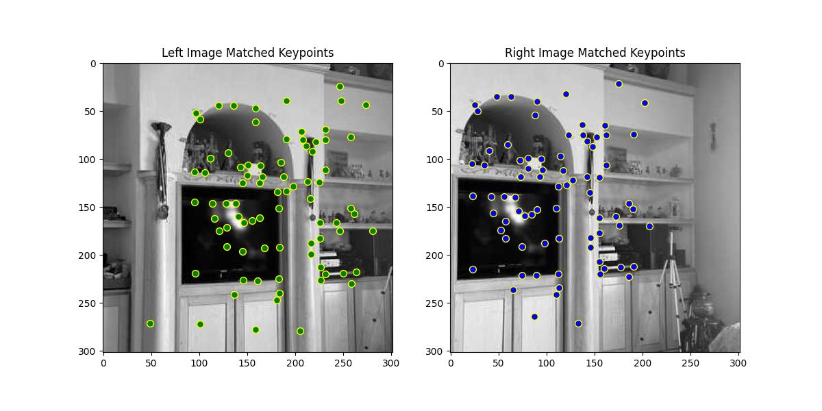
In this step, I perform feature matching between two sets of feature descriptors extracted from two images. Feature matching helps establish correspondences between keypoints in different images, which is crucial for tasks such as image alignment, homography estimation, and 3D reconstruction. The matching is based on the 1-NN/2-NN ratio test proposed by David Lowe, which compares each descriptor with its closest and second-closest neighbors.
Key Steps in Feature Matching:
-
Computing Distances Between Descriptors:
The function computes the Euclidean distance between each descriptor in
Descriptors1and every descriptor inDescriptors2using thedist2()function. The distance metric provides a measure of how similar two descriptors are, with smaller distances indicating higher similarity. -
Finding the Two Nearest Neighbors:
For each descriptor in the first image, the distances to all descriptors in the second image are sorted. The closest descriptor (1-NN) and the second-closest descriptor (2-NN) are identified based on the sorted distances.
-
Ratio Test:
The ratio test compares the distance to the closest neighbor (1-NN) with the distance to the second-closest neighbor (2-NN). The ratio is computed as:
ratio = sqrt(dist_1NN) / sqrt(dist_2NN)If the ratio is less than the specified
ratio_threshold(typically 0.8), the match is considered a good match, indicating that the closest neighbor is significantly better than the second-closest one. This helps reject ambiguous or incorrect matches.
RANSAC
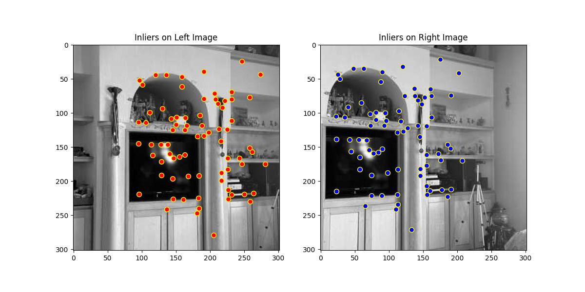
In this step, I use the Random Sample Consensus (RANSAC) algorithm to compute a robust homography between two sets of matched points from different images. RANSAC is used to eliminate outliers (incorrect matches) and retain only the inliers (correct matches), resulting in a more accurate homography estimation. Homography is a transformation that maps points in one image to corresponding points in another image, which is essential for tasks like image stitching and alignment.
Key Steps in RANSAC for Homography Estimation:
-
Random Sampling:
In each RANSAC iteration, the algorithm randomly selects four point pairs from the matched points. These point pairs are used to compute a candidate homography.
-
Homography Computation:
Using the sampled point pairs, a homography matrix
His computed. -
Applying the Homography:
Once the homography matrix
His computed, it is applied to all points in the left image to transform them into the right image. -
Normalizing the Transformed Points:
After applying the homography, the transformed points are normalized by dividing by their homogeneous coordinate to convert them back to Cartesian coordinates (x, y).
-
Reprojection Error Calculation:
The reprojection error is computed as the Euclidean distance between the projected points (transformed using the homography) and the corresponding points in the right image. The error is calculated for each point to determine how well the homography maps the points.
-
Identifying Inliers:
Points whose reprojection error is below the
ransac_threshare classified as inliers. These are the points that fit the estimated homography well and are likely to be correct matches. -
Retaining the Best Set of Inliers:
If the number of inliers found in a given iteration is higher than the previous best iteration, the current set of inliers is saved as the best result. The final output of the RANSAC process is the set of matched points (left and right) that are classified as inliers.
This final set of inliers is used to create a new Homography matrix which is then used to create the mosiacs as in the part A.
Comparison of Automatic vs Manual Stitching
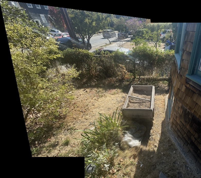
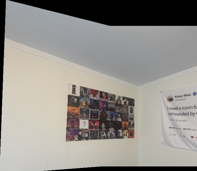
Below we will compare the Manual Mosiacs with the Automatic Mosaics.
My Front Yard

My Room

My Living Room
